# count rows in file
wc -l IVE_tickbidask.txtPractical Implementations for Advances in Financial Machine Learning: Data
Python
Quantitative Finance
Data
Introduction
Data is why data science and quantitative analytics exist! So what good is reading about financial machine learning without some practice on actual data? In this blog post, I document the data (and processing) I used for the modeling and practical exercises one encounters in Advances in Financial Machine Learning by Marcos Lopez de Prado.
Since this whole series of posts on the book’s chapters is a learning exercise for me, I did what anyone who doesn’t know much would do: cheat and trawl Github to see what others have done. This means that I can not pass off the code written here as original. Although I wrote all the code in these blog posts myself (this is a learning exercise after all), I drew heavy inspiration from the work others have already done and provide links to sources accordingly. Whenever our code looks exactly the same, it means that it is still standard practice to code that way.
In particular, this repository by Fernando de la Calle Silos was of great help in shaping my approach. It contains his answers to the exercises in the book, as well as references to free data one can use. To be clear, my intention is not to regurgitate solutions to the exercises in the book. My goal with this data and code is to practically illustrate the math and concepts that Marco addresses in a way that makes sense to me. So with the appropriate dues paid (according to me anyway), let us get into the data.
Kibot
Kibot provides “minute-by-minute intraday data and over 14 years of tick-by-tick (including bid/ask) historical market data for Stocks, ETFs, Futures and Forex.” Although you can purchase data from them, they also conveniently offer a free sample that would suffice for the purpose of practical illustration and practice. On their Free historical intraday data page, they have links to samples for data quality analysis. We go for the S&P 500 Value Index adjusted bid/ask data. More info on the structure of the data file can be found here.
Examine the file
Before I even touch the file with python, I usually prefer to understand more about nature the contents of the file. While python’s data reading capabilities are excellent, we can give it information to read in data more efficiently, and therefore at a faster pace. I will have a blog post with more detail on evaluating raw files in the near future. For now, I just supply the code for Linux bash for ineterest’s sake:
10710652 IVE_tickbidask.txt# what type of file is it?
file IVE_tickbidask.txtIVE_tickbidask.txt: CSV text# see the first couple of lines in your file
head IVE_tickbidask.txt09/28/2009,09:30:00,50.79,50.7,50.79,100
09/28/2009,09:30:00,50.71,50.7,50.79,638
09/28/2009,09:31:32,50.75,50.75,50.76,100
09/28/2009,09:31:32,50.75,50.75,50.76,100
09/28/2009,09:31:33,50.75,50.75,50.76,100
09/28/2009,09:31:33,50.75,50.75,50.76,100
09/28/2009,09:31:33,50.75,50.75,50.76,100
09/28/2009,09:31:33,50.75,50.75,50.76,100
09/28/2009,09:31:33,50.75,50.75,50.76,100
09/28/2009,09:31:33,50.75,50.75,50.76,100Just taking a quick look beforehand reveals quite a bit of helpful information:
- The file contains more than ten million rows so might take a bit of time to read in data.
- The file extension may be
.txt, but it takes on a CSV format. - Printing a sample of the data reveals that the columns in the files don’t come with headers/names, and that I would have to supply these.
- The structure of the data appears to coincide with the description given on the website.
- I now have an idea of data types of each column I want to use.
Some of the information here will help me tell pandas.read_csv() how the data is structured and what I want the format to be like in my dataframe to be. This means python spends less time making educated guesses about the data I am giving it. In turn, less guessing decreases loading time.
Read in the data
Armed with the above information, let’s read in the data and perform some basic manipulations. We want to read in the data, combine the date and the time into one column with a datetime format. We also take the opportunity to create a dollar_volume for later use. Finally, we drop unnecessary columns and clean up a little.
import numpy as np
import pandas as pd

# read the data
df = pd.read_csv(
    'path/to/IVE_tickbidask.txt',
    header=None,
    names=['day', 'time', 'price', 'bid', 'ask', 'vol'],
    engine='c',
    dtype={
        'day':str,
        'time':str,
        'price':np.float64,
        'bid':np.float64,
        'ask':np.float64,
        'vol':np.int64
    }
)

# perform some preliminary manipulations
df['datetime'] = pd.to_datetime(df['day'] + df['time'], format='%m/%d/%Y%H:%M:%S')
df['dollar_vol'] = df['price']*df['vol']
df = df.set_index('datetime').drop(columns=['day', 'time'])

df.head()| price | bid | ask | vol | dollar_vol | |
|---|---|---|---|---|---|
| datetime | |||||
| 2009-09-28 09:30:00 | 50.79 | 50.70 | 50.79 | 100 | 5079.00 |
| 2009-09-28 09:30:00 | 50.71 | 50.70 | 50.79 | 638 | 32352.98 |
| 2009-09-28 09:31:32 | 50.75 | 50.75 | 50.76 | 100 | 5075.00 |
| 2009-09-28 09:31:32 | 50.75 | 50.75 | 50.76 | 100 | 5075.00 |
| 2009-09-28 09:31:33 | 50.75 | 50.75 | 50.76 | 100 | 5075.00 |
Let’s take one last peak at the structure to make sure all is as it should be.
df.info()<class 'pandas.core.frame.DataFrame'>
DatetimeIndex: 10710652 entries, 2009-09-28 09:30:00 to 2023-03-22 16:00:01
Data columns (total 5 columns):
# Column Dtype
--- ------ -----
0 price float64
1 bid float64
2 ask float64
3 vol int64
4 dollar_vol float64
dtypes: float64(4), int64(1)
memory usage: 490.3 MBData checks
We need to ask some questions about the data.
Are there duplicates?
dup = df[df.duplicated()]
dup.head()| price | bid | ask | vol | dollar_vol | |
|---|---|---|---|---|---|
| datetime | |||||
| 2009-09-28 09:31:32 | 50.75 | 50.75 | 50.76 | 100 | 5075.0 |
| 2009-09-28 09:31:33 | 50.75 | 50.75 | 50.76 | 100 | 5075.0 |
| 2009-09-28 09:31:33 | 50.75 | 50.75 | 50.76 | 100 | 5075.0 |
| 2009-09-28 09:31:33 | 50.75 | 50.75 | 50.76 | 100 | 5075.0 |
| 2009-09-28 09:31:33 | 50.75 | 50.75 | 50.76 | 100 | 5075.0 |
It looks like there are quite a number of duplicate rows. Let’s get rid of them:
df.drop_duplicates(inplace=True)Are there missing values?
df.isna().sum()price 0
bid 0
ask 0
vol 0
dollar_vol 0
dtype: int64It looks like there are no missing values.
Are there outliers?
To test for price outliers we’ll take a look at a box plot and then use the mean absolute deviation and the modified z-score to weed these out.
import seaborn as sns
%matplotlib inline

sns.boxplot(df['price'])
<Axes: >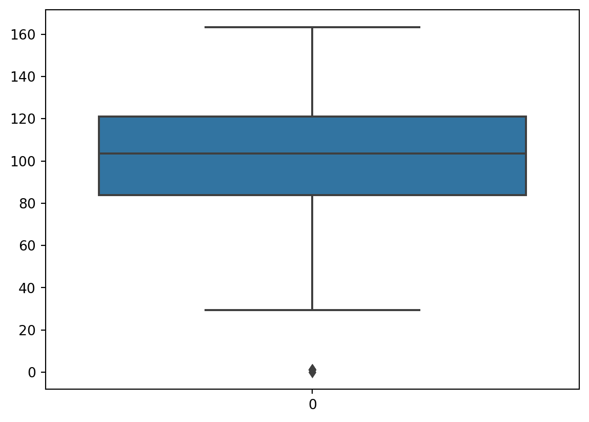
It seems like there are a couple of rows with a price of 0, which is nonsensical. Let’s isolate the price series and go to work on it as an array. Mechanically, we calculate the modified z-score and check whether it is above 3. We construct a boolean array that we then use to remove outliers.
y = np.expand_dims(df.price.values, axis=1) # creat a vertical array (array of arrays)
median = np.median(y)
sum_diff = np.sum((y - median)**2, axis=-1)
abs_diff = np.sqrt(sum_diff)
mad = np.median(abs_diff)

mod_z = 0.6745 * abs_diff / mad # calculate modified z-score

outliers = mod_z > 3. # threshold set at 3 as a float
outliers.sum() # how many observations are seen as outliers?11Let’s remove the outliers:
df = df.loc[~outliers] # ~ reverse the boolean to the opposite (think not outliers)

sns.boxplot(df['price'])
<Axes: >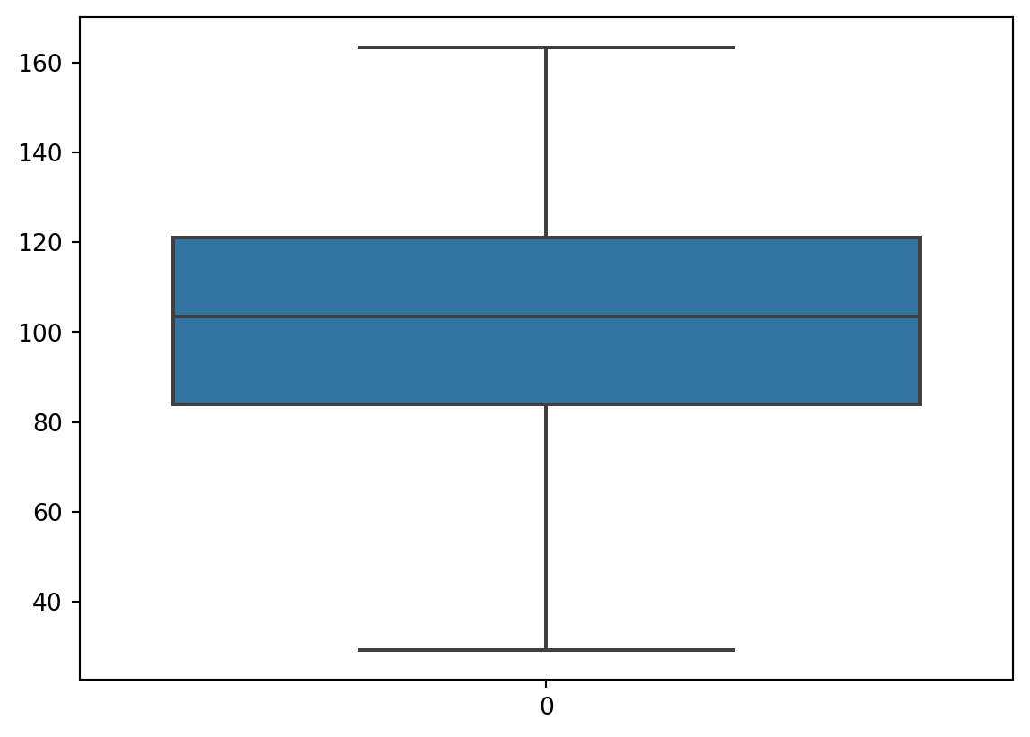
Export Data
The curated data now seems to be in a form that we can trust and work with it. The last step is to export the data to a format that is easily and quickly imported for analysis and practice in the chapters of the book. I settle on parquet, mostly because Fernando uses it in his work and it works really well.
df.to_parquet('path/to/data/clean_IVE_tickbidask.parq')